Essay #10: Four Methods for Computing Weighted Least Squares (WLS) in Python 3
Plus! LaTeX, Gilbert Strang, and musings on intuition.

Motivation: Avoid Rolling Windows
The great workhorse of statisticians and data scientists continues to be the least squares model. It is a natural choice, because analysts are typically called upon to determine how much one variable will change in response to a change in some other variable.
A common follow-up question is how a model’s weights change with time. For ordinary least squares (OLS)1 models, frequently2 this is answered is via rolling windows, and the biggest criticism of such rolling windows is that all data points of the rolling window are weighted equally.
Weighted least squares (WLS) allows us some flexibility to systematically give more weight to more recent data.
If you’re confident about the decay rate & half-life3 of your weighting scheme, then choosing a window length via WLS doesn’t matter — longer dated observations are simply assigned a de-minimis weight.
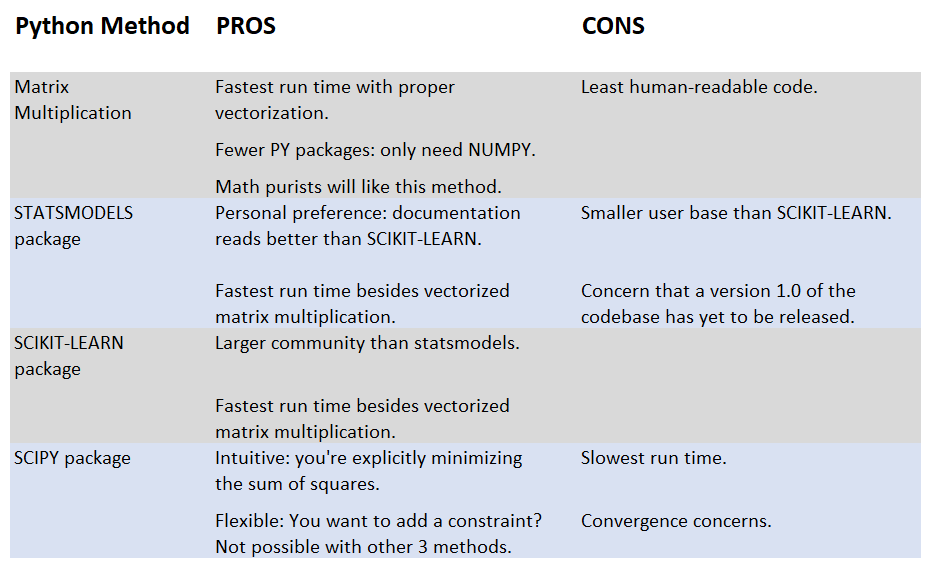
Everyone’s brains work differently; of all the possible ways to do WLS in python, I personally find using SciPy’s minimize method to be the most intuitive, as we’re explicitly minimizing the weighted sum of regression residuals’ squares…hence “least squares”. Of course, each implementation has pros and cons.
Pros & Cons of 4 Python Methods
Sample Code of 4 Python Methods
The test case in all of the above 4 methods is a problem familiar to many folks who have dabbled in financial markets: estimate an asset’s beta, and do so every day.
The two predictor variables are the daily returns of the exchange traded funds SPY & TLT, commonly viewed as proxies of the US stock market & long-dated US Treasury bonds.
I create a synthetic4 response variable with known weights from the two predictor variables, so as to allow us flexibility to investigate how quickly WLS & OLS can retrieve the correct known weights.
For each day from 2011-2019, the response variable is constructed as S% of the daily return of SPY, plus T% of the daily return of TLT, where:
S% = The ones digit of the year (so: 10% in 2011, 20% in 2012, 90% in 2019).
T% = 0% if during the 1st half of the year (Jan 1 - June 30); 50% if during the 2nd half of the year (July 1 - Dec 31).
Each WLS py script applies an exponential weighting scheme: observation t-1 is given 80% of the weight of observation t. For comparison, OLS examples for all 4 methods using a 30-day5 rolling window are included in the GitHub repository.
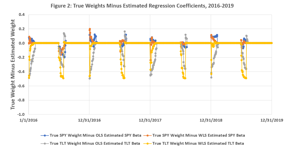
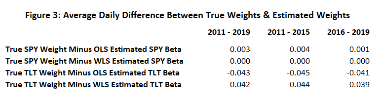
Figures 1-3 below, presented without analysis6, summarize 4 differences:
True SPY Weights Minus OLS Estimated SPY Betas
True SPY Weights Minus WLS Estimated SPY Betas
True TLT Weights Minus OLS Estimated TLT Betas
True TLT Weights Minus WLS Estimated TLT Betas

Commentary
Given:
The matrix of predictor variables: X,
The response vector: y,
The unknown parameter vector of betas: b,
The parameter vector b is computed9 as:
or:
In practice, there are numerous reasons to not use matrix multiplication or a numerical optimizer, especially when other folks have already compiled the StatsModels & SciKit packages! That said, it is still a good idea to check that multiple methods give the same solution.
In experimenting with scipy's minimize function, there are convergence concerns. The default value for the parameter "tol" (tolerance) does not give satisfying precision; while the first 3 python methods have agreement to the 8th decimal digit, using the default "tol" parameter value only gives agreement to the 4th decimal digit. As WLS_2var_method4_scipy.py shows, you will be tempted to tinker with the "tol" parameter to get more precise answers. Unfortunately, increasing the required precision will increase your solution’s run time.
Between StatsModels & SciKit, which would I choose to use in practice? Both packages’ run times are sufficiently fast for most exploratory research purposes. I’d give the tiebreaker10 to SciKit for having a larger userbase.
Appendix A: Version Control / GitHub
Any code, data, and other artifacts produced for this essay are saved here.
Appendix B: Footnotes
The ordinary least squares (OLS) problem is to solve Xb = y, where X is a [t x n] matrix, containing n predictors and t observations. Similarly: y is a [t x 1] vector, and b is a [n x 1] vector of parameters to be estimated.
The verb “estimated” is important here: math purists will want to remind me that the computation of b is an estimation, not an actual solution, as the matrix equations Xb = y represent a system of t linear equations with n unknown variables, typically with t much larger than n, thus yielding no exact solution. Hence the “hat” symbol above the variable b in the LaTeX-formatted equations. Throughout the rest of this essay I will loosely interchange the terms {“estimate”, “solve”, “compute”} and hope that the meaning is obvious from context.
The weighted least squares (WLS) problem is to solve WXb = Wy, where W is a [t x t] diagonal matrix of weights. Many textbooks, including Gilbert Strang’s Introduction to Applied Mathematics, will frame a matrix product W’W as containing the weights; this essay does the same.
We’ll always assume, unless stated otherwise, that the matrix X includes a constant (intercept) term.
I'm not going to argue for e.g. lambda = 0.80 as a better choice than, say, lambda = 0.90 in the sample code to follow. For an example of such explorations, see here.
In the GitHub code snippets I'll call this variable "Frankenstein" or "Frank" or "FrankZ".
30 business days, to be precise.
There is a lot going on during the 2011-2019 sample. To state the obvious, the spikes in the plots are when the weights change (see the earlier definition of “Frankenstein”) and it’s interesting to see how quickly each method “catches up” to the true weights. Figure 3 tells us that this particular implementation of exponentially weighted least squares will usually “catch up” faster than a 30-day window of OLS, but not always.
Stock-bond correlation (and volatility) varies throughout the sample period, which is one reason why the spikes are not the same at the beginning of each half year.
I could have chosen an easier example, but these are the sorts of examples that interest me (and motivated this essay's exploration in the first place).
Off-diagonal terms would indicate that measurements are not believed to be independent. For daily frequency financial data (such as the examples considered in this essay), non-independence is very likely to be present; thus it is also worth running the same regressions on lower frequency data (e.g. 2-day returns, weekly returns). Speaking as a former mathematics grad student: for the absolute best explanation of weighted least squares, including how off-diagonal entries of W generalize to the almighty Kalman Filter, see Section 2.5 of this.
As indicated in footnote 1, the matrix product W’W contains the weights.
Apologies if the LaTeX does not render; it renders correctly for me on Chrome and Firefox, but not Safari. Also renders correctly on the Substack app.
My personal preference (as of 2023) is to give statsmodels the tiebreaker since there is no direct way to compute p-values in scikit-learn.